

Appendix 11: 'Pay for Results’ – Statistical and Mathematical Modeling for Fee Calculations
© 2014 By Dr. Grant McFetridge

11.0: Chose a Fee Method
11.1: Make Choices About Your Practice
11.2: Measure Your Performance
11.3: Calculate a Standard Flat Fee With a Fixed Cutoff Time
11.3.1: Determining the statistically optimum cutoff time C
11.3.3: Determining cutoff time C based on measurements
11.3.4: Determine the flat fee formula parameters
11.3.5: Compute your standard flat fee F
11.3.6: Sensitivity of the fee to variations in parameters
11.4: Calculate a Variable Fee With a Fixed Cutoff Time
11.4.1: Determine parameters for the variable fee formula
11.4.2: Compute your variable fee Fv
11.5: Calculating a Variable Fee With a Variable Cutoff Time
11.5.1: Determine parameters for the variable fee/variable cutoff time formula
11.5.2: Compute your variable fee Fi
11.6: Calculating Fees Based on Estimated Financial Risk
11.7: Calculating Fees Based on the Number of New Clients
Chapter 3: 'Pay for Results'
Appendix 2: Examples of 'Pay for Results' Contracts
Appendix 10: 'Pay for Results' - Fee Calculation Guide
To download a PDF version of this article, right click here.
This appendix is a companion to the simplified therapist fee calculation guide in our Subcellular Psychobiology Diagnosis Handbook (or online at www.PeakStates.com). It is written for the mathematically inclined, especially academics; this appendix derives the equations used to determine the statistically optimum cutoff times and fees for various types of billing approaches.
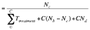
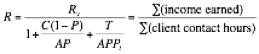
To review, the 'pay for results' fee is derived from a desired ‘equivalent hourly rate’, which makes it compatible with existing billing methods – and makes it simple to understand. Thus:
![]()
11.0: Chose a Fee Method
Now, choose a billing option based on your experience level (or client base) from the list below:
- Appendix 11.3: Compute a fixed per-issue fee that does not vary for any client – the fee is the same no matter how long the job takes. We assume you give up when you reach an upper time limit that is the same for all clients. This is the absolute simplest way of charging and has the least risk for the therapist, but isn't the most cost effective for half your clients. Many ‘pay for results’ therapists use this billing method; it is especially applicable for specialized treatments, such as the Silent Mind Technique™. This formula includes an additional term to cover the non-charged consultation fee.
- Appendix 11.4: Compute a fixed per-issue fee that varies from job to job – the fee is proportional to your estimated length of treatment time. We still assume you give up when you reach an upper time limit that is the same for all clients. Unlike the fixed per-issue fee that doesn't vary from job to job, this charging technique is more economical for the faster half of your clients, but is more costly for the slower half. This billing method is more challenging for the therapist to estimate, so needs a more experienced therapist, and has more financial risk for the therapist. The formula includes an additional term to cover the non-charged consultation fee.
- Appendix 11.5: Compute a fixed per-issue fee that varies from job to job – the fee is proportional to your estimated length of treatment time. However, unlike 11.3 or 11.4, you now give up when you reach your estimated time plus a fixed overrun time. It is useful if your client time estimates are unusually long or widely varying (for example, if you do treatments that typically take 8 hours or more). This billing method poses the highest risk to the therapist, and so needs the most experience. We don’t normally recommend it for most therapists. This formula includes an additional term to cover the non-charged consultation fee.
- Appendix 11.6: Decide if you want to increase your fee for clients that you think will take longer to heal, in order to minimize your financial risk, and to reduce the cost for clients that take less time. However, this is difficult to compute and we don't recommend it for most therapists.
- Appendix 11.7: How do you compute fees if you have a less than a full caseload? We calculate how many new clients you need per week to meet your financial target based on the minimum fee, and then how much to adjust your fee if you have less than optimum numbers of new clients.
11.1: Make Choices About Your Practice
11.1.1: Estimating Your Client Contact Hours (W)
As a therapist with a private practice, you need to decide how many client hours you want to do per week. You also have to account for time you have to spend on the business (making calls, appointments, advertising, chatting with potential organizations, keeping records up to date, billing insurance, paying bills, etc.) If you work a full 8-hour day, it is reasonable to assume 2 hours a day for the other tasks.
Time off is another issue. You need time off, and the clients often don't come in during certain periods of the year. For example, summer months and the month after Christmas are unlikely to have a full caseload. Thus, although it varies widely, the most you can probably expect is 10 months of full-time work at 30 hours per week of patient contact time, and 40 hours per week total work time. This gives a maximum of 1,320 contact hours - and more likely you'll have a lot less contact hours, because you probably won't have a continuous back-to-back stream of clients. Figuring on a half-time caseload is probably a reasonable maximum estimate (although it may be a lot less especially when you start out). With this estimate, you'll only have 660 client-contact hours per year doing private practice (with another 220 hours for other tasks). This number is low for a therapist employed at a facility, but probably realistic for a therapist in private practice.
11.1.2: Determining Your Equivalent Hourly Rate (R)
With ‘charge for results’ you set a price per job, rather than charge by the hour. However, averaged over a number of clients, you can look at your income as if you had a job paying an equivalent hourly pay rate R – the total money you’ve earned divided by the total time you’ve spent with all your clients (i.e., $/hr). This idea is helpful in several ways. It lets you compute fees based on the pay rate you want; allows you to compare your income to those of other therapists; and gives you an easy way to figure out your annual income.
First, you can choose your equivalent hourly rate R by comparing yourself to other ordinary therapists’ hourly rate. Find out what psychotherapists in your area are charging (both the low end and the high end). You then decide where your skill level and your ability to connect to people put you on the local hourly pay range. (Often, being able to make people feel good about themselves and their relationship with you is more important to being able to charge higher fees than being competent in healing clients). Once you have a figure, find out if it meets your annual financial targets - compute what you'll earn at the end of the year to see if it is enough.
The second way to choose your equivalent hourly rate R is to start from the annual income you want, and then compute what you have to charge to meet that target. Obviously, there is some give and take on this - you'll want to find out what the typical range of fees in your area is, so you can see if what you want is reasonable.
According to a 2009 American Psychological Association survey, the median income for a licensed Master’s level in private practice in clinical psychology was $40.5K (SD=27K); for an average of 660 client-contact hours, this means R=$61/hr. The median income for a Masters level in private practice in counseling psychology was $55K; for an average of 660 client-contact hours, this means R=$83/hr. There was also quite a variation of income based on years of experience.
Whatever rate you choose, remember that you offer your general clients two exceptional features that make your services far more valuable than those of your colleagues. First, your ‘charge for results’ policy removes the client’s financial risk. This is the single most valuable thing you can offer a client (especially ones with chronic problems where they have wasted their usually very limited savings in futile attempts to be healed). Secondly, your skill with subcellular psychobiological techniques means that you can help many typical therapy clients who are suffering greatly and cannot get help anywhere else.
- Example 11.2: What should my equivalent hourly rate be?
Because your practice is new, you decide that your base rate should be in the middle of the range of psychotherapy fees in your area. This turns out to be $80/hr. If you figure a half-time caseload and the same average equivalent hourly rate R of $80 per hour, you can expect a gross annual income of $80/hr x 660 hrs = $52,800.
Instead, if you decide that you want an annual income of $100,000 (which is unreasonably high for most general practice therapists, but more possible for therapists who specialize), you'll have to charge an equivalent hourly rate R of $100,000/660hrs = $151 per hour. However, since you're offering very effective therapy with a 'charge for results' policy, you may be worth it - but it will take some time to get you well enough known for this fact to make a difference to your client base.
11.2: Measure Your Performance
To make a fixed-fee, charge only for results process work, you need to know when to quit and accept that you can’t help your client. In a sense, you have an ‘all or nothing’ gamble with each client. At some point your likelihood of success becomes slim; any more time you spend will be unlikely to heal your client or earn you your fee. This appendix applies this idea in different ways (sections 11.3 to 11.6) to trade off risk, client fees, and success rates.
All of the different approaches in this appendix use parameters that you can guess values for, in order to compute your fees. However, it is far better to actually measure key parameters. This lets you select a more optimum cutoff time C that maximizes your income while minimizing your fee, making you as competitive as possible. This value of C also makes your income the least sensitive to parameter variations – this means your gross earning will stay about the same even though your measurements might not be perfectly representative, or your clients have some kind of weird non-normal (in a statistical sense) treatment time probability distribution, or you are sloppy about when you actually cutoff therapy with real clients who you can’t help.
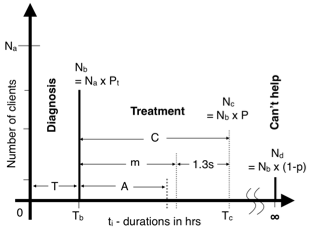
Figure 11.1: Terms in the formulas can be better understood by looking at a frequency distribution plot.
Measure real treatment times and client numbers:
The following procedure usually gives reasonable parameter estimates. (The measurements just help you to roughly figure out the cheapest fee that gives you the most money with the least financial risk. Later, you’ll keep ongoing track of your income and client hours, and make adjustments to your fee or cutoff time as needed.)
During the diagnosis phase you record how many clients (Na) you needed to interview to get 10 healed therapy clients (ones who you genuinely plan to treat, not ones who you would normally have rejected as unsuitable for treatment). Thus, Na is 10 plus all the ones you didn’t treat plus the ones who you worked on but couldn’t help. Record the total time (Ta) that all those interviews took you (including the ones of clients who continued to treatment).
In the treatment phase you record the total treatment time (excluding the diagnosis time) of each of the 10 clients you actually healed. Of course, you can’t heal everyone, but for the harder clients you should continue trying to heal the difficult cases for at least an hour longer than you would normally. This will give you more accurate results (i.e., a better statistical analysis of your client treatment time probability distribution).
In the ‘can’t help’ phase you record how many treatment failures you had - these are the ones you just couldn’t help – to get to 10 clients who healed successfully.
Tip - don’t forget the ‘rule of three’ time: Because of the not uncommon problem of missed or inadequately healed traumas, therapists generally do follow-up sessions after all symptoms are eliminated to make sure that the issue didn't return. This is usually scheduled for a few days after completing treatment, and then usually a phone appointment after 2 to 3 weeks to recheck the healing. Be sure to include this ‘extra’ time in your session length measurements.
Next, derive the statistical parameters from your measurements:
-
 = average of measured time in hours it takes you to do exam, diagnosis, and set your price on all the clients who walk through your door.
 -
 = percent of clients who decide to continue with you after your examination, diagnosis and estimate (the contract acceptance rate) = (# who continue) ÷ (# attempted). Use decimals, e.g. 80% would be 0.8 in the formulas.
 -
 = mean of all your measured client healing times in hours (except for clients that you can’t heal).
 -
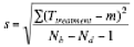 = sampled standard deviation of all your measured client healing times (except for client that you can’t heal). The ideal standard deviation value is close enough if that is the only one your calculator will do.
 -
 = percent of measured clients you could actually heal (given enough time) of the ones you attempted = (# healed irrespective of cutoff time) ÷ (# contracted). Use decimals, e.g. 0.7 means 70%)
- Example 11.3: Measuring parameters
You are concerned about choosing the best C cutoff time that maximize your income R in $/hr. So you start measuring how long your diagnoses and treatments actually take. You keep taking data (and putting in extra time on the slower clients just to see if you can succeed) until you’ve successfully healed 10 clients. Table 11.1 shows your time measurements. Thus, you had to diagnose 15 clients to get 12 that you felt that you could treat (and who wanted treatment). Of those 12, you were able to successfully heal 10 (and that’s when you quit taking data.) You could not heal two of those twelve clients and so they were shown as ∞ in the table (hence p = 80%).
| Tdiagnosis (diagnosis times, minutes) | Tdiagnosis (diagnosis times, hours) | N (number of clients) | T (average time for diagnosis, hrs) | Pt (% of diagnosis clients who you then treated) |
| 25, 35, 40, 26, 37, 22, 40, 28, 38, 15, 17, 50, 28, 40, 20 | = 0.42, 0.58, 0.67, 0.43, 0.62, 0.37, 0.67, 0.47, 0.63, 0.25, 0.28, 0.83, 0.47, 0.67, 0.33 | Na=15 clients in diagnosis Nb=12 clients attempted | T=∑Ta/Na =(0.42+0.58+0.67 +0.43+0.62+0.37 +0.67+0.47+0.63 +0.25+0.28+0.83 +0.47+0.67+0.33)/15 =7.69hr/15clients =0.51 hrs/client | Pt=Nb/Na =12clients/15clients =0.80 (80%) |
| Ttreatmentt (treatment times, hours) | N (# number of clients) | m (mean, without a cutoff) | s (standard deviation, without a cutoff) | p (% healed, without a cutoff) |
| 0.5, ∞, 4.0, 1.5, 2.5, 1.0, 3.0, 1.5, ∞, 2.5, 2.0, 2.5 | Nb=12 clients attempted Nd=2 couldn't heal | m=(∑Ttreatment)/(Nb-Nd) =(21.0 hrs)/(12-2 clients) =2.1 hrs/client | s=√[∑(Ttreat-m)2/(Nb-Nd-1)] =√[9.4/12-2-1] =1.02 hrs | p=(# healed)/ (#attempted) =(Nb-Nd)/Nb =(10-2)/12 =0.83 (83%) |
Figure 11.2: Time data on 15 clients (taken one after another). Diagnosis times were measured in minutes, so had to be converted to decimal hours for the formulas. This therapist got a little lazy and measured the treatment times in increments of a half hour.
You then compute the mean (m) and the sampled standard deviation (s) of your 10 (or more) successful therapy times. Hence, m is 2.1 and s is 1.02 hours. You are now ready to figure out your fee.
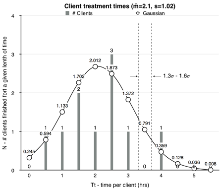
Figure 11.3: A frequency plot of the 10 treatment times (shown as solid bars) for Example 11.3.
A truncated Gaussian curve with the same mean and standard deviation is plotted over the bar graph.
11.3: Calculate a Standard Flat Fee With a Fixed Cutoff Time
In reality, most therapists who use the ‘pay for results’ model simply use a standard, set fee they charge for every ordinary therapy issue. Essentially, "one size fits all". Typical fees for general therapy range around $400US per contract, but vary with country and cost of living.
11.3.1: Determining the statistically optimum cutoff time C
Unfortunately, there is no closed analytical solution for an optimum C (cutoff time) and the derived R (equivalent hourly rate) for every therapist. It varies too much with the therapist’s ability, the types of problems their clients have, the fit of the data points they measured to a (hopefully) real underlying distribution, and the stability of that distribution over time. However, what we can do is plot various types of probability distributions of client times versus C, R and p. Fortunately, from these plots it turns out that we can generate a ‘rule of thumb’ for getting a near optimum value for C by using Gaussian statistics. Once we have that, we check it against the C versus R plot from our measured treatment times to select an optimum cutoff, and then monitor the results over time.
We’ll use the following equation to plot normalized equivalent hourly rate R curves to find an optimum cutoff C. The formula is for a rate RN (normalized for a fee=$1) as a function of cutoff time C for arbitrary frequency probability distribution of treatment times N(t). (We’re ignoring the time spent during diagnosis – that is added on later.)
Eq. 11.1 ![]()
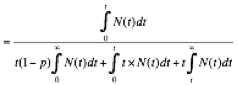
where RN, treat(t)=Rate in $/hr-fee for treatment only (normalized to a $1 fee), IN=Income in $ normalized to a $1 fee, TT,treat=Total client treatment hours, N(t)=probability distribution of client times, p=percent success of treatment clients (ignoring cutoff); all for t=cutoff time C.
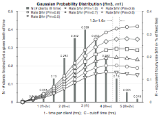
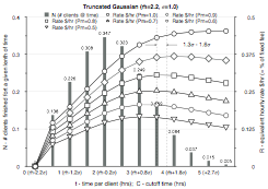
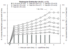
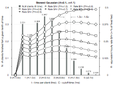
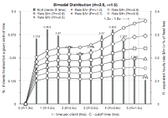
Figure 11.4: Plots of equivalent hourly rate R for changing cutoff C times for various distributions normalized to a fixed fee of $1. Success rate p is varied from 100% to 50% in 10% increments to give a family of curves. The mean plus 1.3 and 1.6 standard deviation values are shown as dashed vertical lines.
Figure 11.4 shows normalized equivalent hourly rate plots for various client treatment time distributions. The best cutoff time C is when the curve of RN reaches a maximum. However, not only does this maximum vary with the client treatment time distributions, it also varies somewhat with the percentage success rate p – a worse success rate means it is more optimum to have a shorter treatment cutoff time.
With statistically derived values for m, s, and p, we can now make a reasonable ‘rule of thumb’ estimate for C, the cutoff time. See the lookup table below on C versus p. (This level of time accuracy is a bit of an overkill, given how sloppy all the approximations are; in real use, therapists just round this C to the closest half hour and use that as a target cutoff time.) You can now compute the smallest fee that still allows you to still meet your financial target – and this increases your likelihood of keeping clients. Assuming a Gaussian distribution of clients, this means you will heal roughly 90% to 93% of them (not counting the ones that you could never have healed anyway).
| p (% success) | C (statistical) | CDF (Gaussian) |
| p=0.9-1.0 | C=m+1.7s | 96% |
| p=0.8-0.9 | C=m+1.5s | 93% |
| p=0.7-0.8 | C=m+1.35s | 91% |
| p=0.6-0.7 | C=m+1.2s | 89% |
| p=0.5-0.6 | C=m+1.1s | 86% |
Figure 11.5: A lookup table for choosing a ‘rule of thumb’ value for C.
A rough approximation for Gaussian or positive skewed (rather than
more rectangular) distributions is s=2.04p-0.13.
11.3.3: Determining cutoff time C based on measurements
Even though you can compute a statistics-derived value for cutoff time C, you should check it against reality. The easiest way is to use your 10 (or more) measured Ttreatment values to make an RN versus C plot. On the plot, you can compare the measured optimum RN with the statistical table RN and choose a final value for C. The best choice is where the hourly rate RN is a maximum. Unfortunately, choosing between the statistical C and the real C is somewhat of a judgment call, since you only have 10 or so measured values that might not be too representative of the real probability distribution - but it does allow you to visually see if there is something obviously off in your statistical choice.
The formula for the normalized hourly rate R as a function of C is:
Eq. 11.2 ![]()
![]()
· RN,treat = equivalent hourly rate (the per-hour rate that you would get if you were just a normal therapist) in $/hr, divided by the fee F to give a normalized value. The effect of diagnosis time is added later. To un-normalize, Rtreat = RN,treat x F (in $/hr).
· C = maximum hours for the client cutoff (i.e., no fee charged after this length of time).
· Nb = # of clients you start treatment with.
· Nc = # of clients you treated up to and including the cutoff time.
· Nd = # of clients that you can’t help.
- Example 11.4: Choose C from the measured data
In Example 11.3 we derived mean (m) and standard deviation (s) for the 10 measured client treatment times (without using a cutoff time). We use the lookup table in figure 11.5 to get a ‘rule of thumb’ value for C. Since m=2.1, s=1.02, and p=0.83, we find:
C = m+1.5s = 2.1+1.5x1.02
= 3.63 hours.
We then visually check our statistical estimate against a plot of the actual data’s hourly income RN as a function of cutoff time C. This gives us a feel for our data’s RN’s sensitivity to the cutoff time C. We use equation 11.2 to make this plot. Because we only had 10 points, the RN curve is not very smooth – the maximum equivalent hourly income is the same for C=3 or 4 hours, but drops 8% for a cutoff time of C=3.5 hours. Thus, since we want the maximum RN, the statistically derived value of C=3.63 hours looks reasonable. True, there is a dip just about the point we are choosing, but if we smooth out the curve by eye, it looks like that is close to the maximum RN value.
| C=0 | C=0.5 | C=1.0 | C=1.5 | C=2.0 | C=2.5 | C=3.0 | C=3.5 | C=4.0 | C=4.5 | C=5.0 | C=5.5 | |
| ∑Ttreat (0 to C) | 0 | .5 | 0.5+1.0 =1.5 | 0.5+1.0 +1.5+1.5 =4.5 | 0.5+1.0 +1.5+1.5 +2.0 =6.5 | 0.5+1.0 +1.5+1.5 +2.0+2.5 +2.5+2.5 =14 | 0.5+1.0 +1.5+1.5 +2.0+2.5 +2.5+2.5 +3.0 =17 | 0.5+1.0 +1.5+1.5 +2.0+2.5 +2.5+2.5 +3.0 =17 | 0.5+1.0 +1.5+1.5 +2.0+2.5 +2.5+2.5 +3.0+4.0 =21 | 0.5+1.0 +1.5+1.5 +2.0+2.5 +2.5+2.5 +3.0+4.0 =21 | 0.5+1.0 +1.5+1.5 +2.0+2.5 +2.5+2.5 +3.0+4.0 =21 | 0.5+1.0 +1.5+1.5 +2.0+2.5 +2.5+2.5 +3.0+4.0 =21 |
| Nc | 0 | 1 | 2 | 4 | 5 | 8 | 9 | 9 | 10 | 10 | 10 | 10 |
| C(Nb-Nc) | 0 | 0.5(10-1) =4.5 | 1.0(10-2) =8 | 1.5(10-4) =9 | 2.0(10-5) =10 | 2.5(10-8) =5 | 3.0(10-9) =3 | 3.5(10-9) =3.5 | 4.0(10-10) =0 | 4.5(10-10) =0 | 5.0(10-10) =0 | 5.5(10-10) =0 |
| CxNd | 0 | 0.5(2) =1 | 1.0(2) =2 | 1.5(2) =3 | 2.0(2) =4 | 2.5(2) =5 | 3.0(2) =6 | 3.5(2) =7 | 4.0(2) =8 | 4.5(2) =9 | 5.0(2) =10 | 5.5(2) =11 |
| RN(C)$/hr =R(C)/F | 0 | 1/(0.5+ 4.5+1) =0.167 | 2/(1.5+ 8+2) =0.174 | 4/(4.5+ 9+3) =0.242 | 5/(6.5+ 10+4) =0.244 | 8/(14+ 5+5) =0.333 | 9/(17+ 3+6) =0.346 | 9/(17+ 3.5+7) =0.327 | 10/(21+ 0+8) =0.345 | 10/(21+ 0+9) =0.333 | 10/(21+ 0+10) =0.323 | 10/(21+ 0+11) =0.313 |
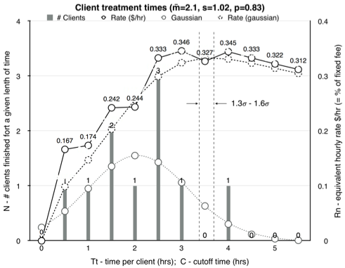
Figure 11.5: Plot of normalized hourly rate RN as a function of cutoff C for the example measured treatment times.
11.3.4: Determine the flat fee formula parameters
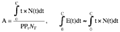
We’re now going to derive the parameters you’ll need to compute your fee and equivalent hourly rate. All the calculations from now on will be on data using a chosen maximum time cutoff – no special test group is needed. Note that this assumes that you have a full caseload – i.e., you have as many new clients as you have time available. If this is not the case, see appendix 11.7.
A = average hours per client with clients you can heal up to the cutoff time. (Exclude the clients past the C cutoff, and exclude the diagnosis time.) A = (total successful client treatment times les diagnosis time) ÷ (# of clients treated successfully).
Eq. 11.3 
P = percent of clients who successfully heal up to the cutoff time, based on the total number of clients you actually do healing work with. P = (#healed up to cutoff) ÷ (# attempted). Exclude clients you diagnosed but did not treat. Use decimal, e.g. 70% would be 0.7 in the formula.
Eq. 11.4 ![]()
Adding for diagnosis time:
When calculating a standard fixed fee, you include your diagnosis/exam time as part of your 'charge for results' fee, not as a separate fee. So you need to increase your standard fee (hopefully not too much) to cover the diagnosis time for clients that contract with you and for ones who end up deciding not to use your services. To figure this part of the standard fee, you will have to determine the average time it takes you to do an examination (T), and the percentage of clients who continue with you after the diagnosis (Pt).
Thus, your success rate (the percentage that you actually heal) for every client who walks in the door is a combination of your skill in diagnosing, luck in getting clients you can actually help, your ability to convince clients to try your services, and your skill in actual treatment:
![]() (in decimal)
(in decimal)
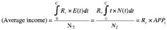
The average time you spend per client on every client that walks in the door is:
Eq. 11.5 ![]()
![]() (in hrs/client)
(in hrs/client)
11.3.5: Compute your standard flat fee F
Thus, the fixed per issue fee F to charge clients is shown below. The first term covers the time spent healing, the second term covers the average diagnosis time.
![]()
Eq. 11.6 ![]() (in $)
(in $)
Your equivalent hourly rate R, if you chose to calculate it from a given flat fee F, is:
Eq. 11.7 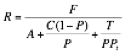 (in $/hr)
In the figure below we illustrate graphically one way that you can use equation 11.6. The ratio of two measured values, average client-contact time and success rate, allow us to easily choose the minimum standard fee for a desired income or hourly rate. Although the term Tave/PPt can be computed from other parameters (eq. 11.6), it is far easier if the therapist just keeps a running total of his client-contact hours divided by how many clients he successfully heals to get (and constantly update) this key value. By monitoring your performance in your practice, you can adjust your client fees as needed to give you your target income or hourly rate (if you have a full client load – if you don’t, see section 11.7).
![]()
Eq. 11.8 ![]()
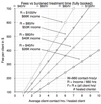
Figure 11.6: Tradeoffs between fee, hourly rate, yearly income, and performance parameters. The x-axis = Tave/PPt.
Example 11.5: Calculate your hourly rate R and your standard fee Fd from your measured data
In Example 11.3 and 11.4, we plotted the data from our measured client session length data and chose C=3.63 hours. We can now compute a fee based on the equivalent hourly rate we want to earn. From example 11.4, we derived the mean time for client interviews at T = 0.51 hrs, and the contract acceptance rate Pt = 0.80 (80%). Now let us say we want an equivalent hourly rate of R = $100/hr.
From equation 11.3,
A = (0.5+1.0+1.5+1.5+2.0+2.5+2.5+2.5+3.0)/9
= 1.89 hours
From equation 11.4,
P = (#healed up to cutoff)/(#attempted) = Nc/Nb
= 9/12
= 0.75 (75%)
From equation 11.6,
F = 100[1.89+(3.63(1-0.75))/0.75] + 100[(.51)/(0.75x0.8)] = 100[3.1] + 100[0.85]
= $310 + $85
= $395 per issue.
As we noted in example 11.4, the curve of RN derived from measured data has a ‘dip’ in it at 3.5 hours that would probably smooth out with more samples. Thus, the fee we compute here is a bit excessive – over time we would expect to earn a little more money than we were planning on (our hourly rate would be more than the target $100/hr). If our clients are unusually price sensitive, we could use accumulated data from more real clients to compute a slightly less expensive fee.
In the ‘pay for results’ model, we don’t charge for time spent on diagnosis if a client decides to turn down a contract, or we decide we can’t help them. We cover this time by increasing our fee slightly – in this case, by $17 of the flat fee amount ($85 x (1-Pt) = $17). (The average paying customer part of the diagnosis fee is $85 x PPt = $51, and the ‘can’t heal’ group’s part is $85 x Pt(1-P) = $17.)
Example 11.6: How much do you earn if you charge with a ‘per hour’ flat rate fee?
Because all of this 'charge for results' stuff is so new to you, you are not willing to ask the client for the real per-issue fee you should charge to meet your financial target. Instead of computing what you need to charge, you decide to just charge using the going rate for therapy - $100/hr in this example. Using the data from example 11.5, your cutoff time C=3.63, you average A=1.89 hours per client for successful treatment and spend T=0.51 hours on average for diagnosis. Thus, you charge your successfully healed client a flat fee of F = $100/hr x 0.5 hrs (for the consultation) + $100/hr x 2hrs (for the healing) = $250. But you are curious to find out what you are really earning after you include time spent on clients you couldn’t help. Thus, from equation 11.7 your average take-home pay (your equivalent hourly rate) would be only:
R = F ÷ {[A + C(1 - P)/P] + [T/ PPt]}
= $250 ÷ {[1.89hr + 3.63hr(1 - 0.75)/ 0.75] + [0.51/ (0.8 x 0.75)]}
= $250 ÷ {3.95}
= $63/hr.
11.3.6: Sensitivity of the fee to variations in parameters
Up to this point, we’ve been just figuring out how to compute the necessary fee given various measured parameters (or assumptions). We’ve worked to pick a cutoff time C where small variations in it don’t affect our equivalent hourly rate (and hence our fee) very much. However, what happens if our averages or probabilities shift? Can we trust that the fee we chose is good enough, or does our income wildly change due to minor shifts in parameters? Do we have to add an extra amount to the fee to keep our income adequate? It turns out that for most people, it makes more sense to use their estimates as is, and simply check their income over time to see if they need to adjust their rates.
Fortunately, we can evaluate this question mathematically. Using sensitivity analysis on equation 11.5, we get equations that give us the approximate percentage change in the fee F due to small percentage changes in a parameter. (For those readers unfamiliar with sensitivity analysis, the ‘sensitivity’ of the fee to changes in a parameter depends on the initial conditions of your system. Thus, you have to plug in your starting values to evaluate your sensitivities.) Conveniently, the sensitivity of the fee F to the rate R (and vice versa) is 1 – for example, a 10% increase in the desired hourly rate will require a 10% increase in the needed fee. This also means that if you hold the fee F constant, your equivalent hourly rate R to the different parameters is the negative of the sensitivity of the fee F to those parameters.
Eq. 11.9 ![]()
Eq. 11.10 ![]()
Eq. 11.11 ![]()
Eq. 11.12 ![]()
- Example 11.8: How much does income change with shifts in your parameters?
Using the values in example 11.5, we can evaluate the sensitivity of the fee (or the equivalent hourly rate) to small changes in parameters. Note that sensitivities depend on the initial conditions. Using equations 11.9-12, for P=0.75, Pt=0.8, T=0.51hrs, A=1.89, C=3.6hrs we get:
∫Sensitivity (% fee F) ÷ (% success rate P) = -1.43
∫Sensitivity (% fee F) ÷ (% hourly rate R) = 1.0
∫Sensitivity (% fee F) ÷ (% average time A) = 0.48
∫Sensitivity (% fee F) ÷ (% cutoff time C) = 0.30
∫Sensitivity (% fee F) ÷ (% probability of treatment Pt) = -0.22
So let’s look at some reasonable variations… (Remember, all of these sensitivity results are approximate!) For a change of +5% to P, your fee could be lowered by -7.2%, or if you leave your fee unchanged, your equivalent hourly income would rise by 7.2%. For a 10% increase in your average treatment time A, your income would drop by about 5%. If your cutoff time C stretched out by 30 more minutes (for your current cutoff time of 3.6 hours that would be a 0.5hr/3.6hr=14% change) which means your income would go down by about 4%. And if get a higher percentage of clients decide to work with you, with Pt increased by 5%, your income would increase by about 1.1%.
What can we expect if our parameter estimates are off by random amounts? In a worst-case scenario, the parameters that you used to set your fee are all off in the wrong direction. Given the variations we just used as maximums, you might expect that your income is about 7.2+5+4+1.1 = 17% lower than you expected! Fortunately, random errors sum statistically using root-mean-squares. Hence, ±√(7.22+52+42+1.12) = ±10%. So you could anticipate that your income would probably be about what you were planning on, but it could be up to a maximum of 10% off in either direction (assuming the maximum parameter variations were as shown in the previous paragraph). If you were a pessimist, you would expect the worse and add 10% to your fee just in case. Most people would just wait to see how it played out in real life, and adjust if needed, since the nominal value will probably be about right.
Now, what would happen if you simply got more competent, and the variations were all due to you getting faster and better? In this case, the percentages all add together in a nice way: 7.2+5+4+1.1 = +17% more income than you were expecting (assuming you also had a full case load). Of course, you could also simply lower your fee by that 17 % to keep your yearly income at the level you were targeting – or just keep the extra for a rainy day.
11.4: Calculate a Variable Fee With a Fixed Cutoff Time
With more experience, you may want to quit using the same fee for every issue. (Although in our experience most clients are fine with the standard fixed fee from section 11.3, because they’re paying you to eliminate their issue, not for your company.) Instead, you estimate how long it should take (E), and offer the client a fee based on your time estimate. You will still put a fixed upper limit C on how much time you're willing to spend with any client, just as in the previous method. (For example, you still quit at 4 hours no matter what. Note that stopping at a fixed time doesn’t abandon the client, because you'll pass them on to a more skilled practitioner.)
This method gives you the ability to tailor your fees to match your expectations of how you should be charging - more for a longer problem, less for a shorter one. However, this method has more inherent financial risk for you, as you’ve now added the uncertainty of how well you can make accurate time estimates. Worse, mistakes in the larger estimates have a much bigger financial impact than with shorter ones. Like gambling, there is also a tendency to go past your cutoff time, trying to get that large payout. And note that you can’t mix variable fees with fixed fees – charging less for shorter work has to be balanced by charging more for longer work.
You need to be skilled enough to recognize when clients have an issue you simply can't handle and screen them out of treatment, to help reduce the inherent financial risk with this method. Obviously, in this approach you will screen some people out, and screen some people in, and get it wrong occasionally. But on average, with practice you should be able to do this and improve your success rate, and so be able to charge the faster client less than with the fixed fee method.
It is very useful to generate a personal list of average times for the different problems you see in clients and place for quick your desk reverence (perhaps notes in the categories in this handbook). Ideally, you would create a handbook of standard times for different problems, as in car repair, and just pre-calculate the price using the client hourly rate you’ve computed.
11.4.1: Determine parameters for the variable fee formula
As in section 11.3, you pre-assign a maximum cutoff C on the number of hours you're willing to work with a client. Your success rate is still P. (P is higher than for a beginner because you are skilled enough to filter out the obviously impossible cases.) Your desired equivalent hourly rate (as if you were a regular therapist) is still R. The average time per healed client is still A. To estimate these parameters, evaluate at least 10 successfully healed clients and compute your estimated average time to completion.
You will also want to keep track of your performance over time. It is important for you to recognize if you have any systemic problems with your estimates (i.e., they're always low, which might become a serious financial problem, or always high which is not a financial problem for you but is for your client and makes your fees higher than necessary and so less competitive).
- R = equivalent hourly rate (the per-hour rate that you would get if you were just a normal therapist) in $/hr. R = (total income) ÷ (total client contact-hours).
- A = average hours/client with clients you can heal (exclude the times of ones past the C cutoff). A = (total treatment time of successfully healed clients, excluding diagnosis time)/(# of successfully healed clients).
- P = percent success rate = percent of clients who successfully heal, based on the total number of clients you actually do healing work with. P = (# healed) ÷ (# attempted). Use decimal, i.e. 70% would be 0.7 in the formula.
- C = cutoff time, the fixed length of time when you give up and end treatment, in decimal hours.
- T = average time it takes you to do exam, diagnosis, and set your price, in decimal hours. T=(sum of all diagnosis times) ÷ (# of clients in the door).
- Pt = percent of clients who decide to continue with you after your examination, diagnosis and estimate. Pt = (# who continue) ÷ (# clients in the door). Use decimal, i.e. 50% would be 0.5 in the formula.
In this variable billing method as in the fixed fee method, you still have to quit working with a client whenever your time spent with the client passes a certain fixed time threshold. Obviously, there are many reasons that cause you to have to quit that are totally outside of your control - the particular client doesn’t heal fast enough for your available time, the sheer number of their traumas takes too long, they are unable to successfully use a technique, they are an unusual complicated case, or due to the fact that the state of the art is simply not good enough to heal everyone.
11.4.2: Compute your variable fee Fv
In the variable fee method with fixed cutoff, we need to compute a new term Rv (v for variable), the hourly rate you use to set a client’s fee. This is the rate you will have to charge to get the same amount as if you were just a regular therapist charging a flat hourly rate. Your estimated time for that particular client's issue = Ei (in statistics i is for a list of items). Fi is the amount you charge the client, which varies for each issue: Fi = Ei x Rv. Obviously, this approach is riskier on a per-client basis, because people and their issues can be unpredictable. However, although you may not be able to accurately guess the precise length of treatment with any given client, over many clients your wins and losses will average out.
- Ei = estimate of how long a given client's issue will take to heal in hours (based on your experience)
- Rv = customer specific rate, in $/hr that includes diagnosis time (answer you are calculating)
- Fi = Variable per-issue fee in $ for a particular issue that includes diagnosis time (answer you are calculating)
Computing the amount you are going to charge is straightforward after you've figured out your average numbers. Since most therapists will work with clients in increments of 30 minutes (i.e., an office visit might be 1.5 hours long), you can have a table of fees based on 30 minute break points.. The only proviso is that you really stop when the client is finished - you don't just keep talking to fill up the rest of the client's hour. If you do plan on just chatting to fill up time on a regular basis, you'll need to compute your average time A to reflect this fact so you bill appropriately.
Thus, to calculate the variable per-issue fee Fi for a particular client issue:
Eq. 11.13
Your hourly rate Rv to charge clients (the second term in 11.15 is for diagnosis time) is:
Eq. 11.14
Eq. 11.15
Your equivalent hourly rate R, if you chose to calculate it from your fee rate Rv, is:
Eq 11.16
 (in $/hour)
You need to monitor your income over time to see if your fees continue to give you your expected equivalent hourly rate (or yearly income) R. This is simply the total income divided by the total client contact hours. If this is not meeting your expectations, you need to scale your customer specific rate by the same percentage.
For math geeks only: Because we're assuming that you've done a good job on estimating the average job times (i.e., the time that your faster clients take exactly balances the time your slower clients take), over reasonably large numbers of clients the sum of your estimated times is (hopefully) equal to the sum of the actual times. Only the clients that exceed your time threshold and don't get charged matter in our formula derivation, and is accounted for in the measured average failure time. To compute a formula for Rv, we note that the average time is a scaled version of the average income, and nicely accounts for any particular client probability distribution.
You can also compare the equivalent flat fee against your variable fees. The assumption that the integral of your time estimates equals the integral of your actual distribution of healed client times means that the derivations in section 11.3 still apply, thus:
- Example 11.9: Compute a client hourly rate for your variable fees
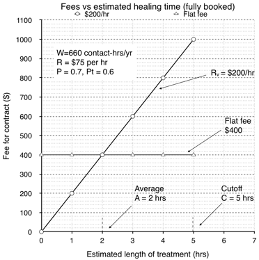
In this example you're now charging each client differently depending on your time estimate for that client. Thus, an experienced therapist will take about 30 minutes to take a history, diagnose, set criteria for results, and set a price, so T = 0.5 hours. Let us arbitrarily assume that 60% of the clients in the door decide to take a chance with you, so Pt = 0.6 (60%). Your equivalent hourly rate R target is still $75/hour, your cutoff C is 5 hours, your success rate P is 70%, and your average time per client A is 2 hours. (Thus for every 100 clients who walk in the door, 60 clients start therapy and 42 successfully heal.) Thus,
Rv = 75 x [1+ (5(1 - 0.7) ÷ (2 x 0.7))] + 75 x [0.5 ÷ (2 x 0.7 x 0.6)]
= $155 + $45
= $200 per hour.
The number of clients you need to see per year is from equation 11.18: NY=660hrs/yr ÷ Tave = 660/2.24 = 294 clients per year. This means about 294/43.4 = 6.8 new clients per week.
After you compute the rate that you need to charge, you wonder what your income would be if you just charged the going rate for therapy (at $75/hr in this example). Then your average take home pay would be only R = $75 ÷ 2.667 = $28/hr.
And finally, you wonder if billing like this makes sense. Remember, you don’t get to reduce your top fee (because it is extremely high), otherwise you won’t make your income target. So you compute the fixed flat fee amount you’d have to charge (using equation 11.6), and it comes out to be $400 for any client. In this particular example, for many of your clients the flat fee would seem like a real bargain!
11.5: Calculating a Variable Fee With a Variable Cutoff Time
In this fee method you would still estimate how long it was going to take to treat your client to set your price. However, rather than stopping at a fixed cutoff time C (say 6 hours from the start of therapy), you add the cutoff time to the estimated time. We call this added cutoff time the upper limit L.
For example, you have a client you think will take about 4 hours. In the flat fee method of section 11.3, with a cutoff of 6 hours you would quit at 6 hours no matter what. In this variable fee/variable cutoff approach, if the upper limit L was 3 hours, then you would go your estimated time of 4 hours, then continue for another 3 hours after that for a total of 7 hours and then quit (if unsuccessful in healing).
This fee method is not recommended for general practice therapists due to the high financial risk - it is much easier to lose money this way than with the previous methods. If you made a high estimated time to heal (E) and didn’t succeed, you’ve lost a proportionally larger part of your revenue than the other fee methods give. Too, as general practitioners our client times are relatively short - the fixed fee, fixed cutoff method would usually work fine. As with the method in section 11.4, if we do choose this method, it is helpful to accumulate a manual of average times for various problems so you can quickly do estimates for clients. For example, you could enter standard times in this handbook. Unfortunately, a general practitioner usually sees a huge range of problems making it a lot harder to create a set of standard times. Since you can have clients go to more advanced therapists to handle the longer, more difficult cases this billing method is even less attractive. Most therapists have an arrangement with a more skilled therapist (generally an Institute clinic therapist) to share some of the fee if they successfully heal your client.
The one case this method might be useful is for specialists, where they have a limited number of processes and can predict their times well. This can give them more flexibility with clients - they can plan on working much longer with a given client, instead of running into the fixed cutoff time C. Unlike general practitioners, specialists work with a more limited set of problems, so making a standard time manual is much more reasonable.
11.5.1: Determine parameters for the variable fee/variable cutoff time formula
Most of the variables we’ll use with this method are the same as with the flat or variable fee with a fixed cutoff (sections 11.3 and 11.4). We still measure the average time A that it takes to heal our clients. P is still the percent of clients that you successfully treat, and so on. Thus:
- R = equivalent hourly rate (as if you were just a normal therapist charging by the hour) in $/hr.
- A = average hours/client with clients you do heal (exclude the times of ones past the C cutoff). A = (sum of times for healed clients) ÷ (# of healed clients).
- P = percent of clients who successfully heal, based on the total number of clients you actually do healing work with. P = (# healed) ÷ (#attempted). Use decimal, i.e. 70% would be 0.7 in the formula.
- T = average time it takes you to do exam, diagnosis, and set your price.
- Pt = percent of clients who decide to continue with you after your examination, diagnosis and estimate = (# who continue) ÷ (# all in the door). Use decimal, i.e. 50% would be 0.5 in the formula.
The new terms are:
- Rvc = hourly rate to set contract fees with.
- AL = average time for clients who we can't heal. AL = (total time of failures) ÷ (# of failures).
- Ei = estimate of how long a given client's issue will take to heal in hours (based on your experience).
- L = upper limit to the time we work on clients. It is added to the estimated treatment time to establish a cutoff time to stop working on the client. Choosing L is an iterative process – start with L ≤ C from the fixed fee billing method (see section 11.3).
11.5.2: Compute your variable fee Fi
The fixed fee you could offer while still using this method of time estimation and fixed additional cutoff L is:
The average per hour fee Rvc (includes diagnosis fee) is:
Eq. 11.17
If you choose to offer a fixed fee F using the variable time, variable cutoff method, it is:
If you choose to offer a variable per issue fee Fi (includes diagnosis fee), it is:
The variable fee/fixed cutoff equations of section 11.4 were modified by noting that the average time for clients we were not able to heal AL acts as if it were a cutoff time C. However, the confidence that you can compute an accurate fee is considerably lower, because the average AL has a high standard deviation. Note that both Ei and L are not used in the computation of the equivalent hourly rate R - instead, the therapist estimates E for a given client, notes it down, and quits working if the additional time limit L is exceeded.
The therapist needs to keep a running tally on his income and client hours to make sure his equivalent hourly rate is being met (or equivalently his yearly income target). You scale Rvc by the same percentage to compensate.
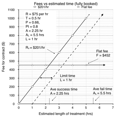
- Example 11.11: Calculating a client hourly rate for the variable fee/variable cutoff method
We've chosen to forfeit our fee if the treatment takes 1 hour longer than we anticipated (L=1). However, note that this number has no effect on the calculation, because this information is contained in the average time we spent on clients who were not successfully healed. If, for example, we were to decide we were too inflexible, we would have to compute new averages and re-compute the fees we had to charge. Let us say we had an A of 2.25 hours, and an AL of 5.5 hours. Let us also say we had a P of 66% (i.e., 0.66), and Pt = 0.8, and T = 0.5hrs. Our base rate R is still $75/hr. Thus, Rvc would be $201/hr.
Instead of computing what you need to charge, you decide to just charge the going rate for therapy at $75/hr in this example. Using equation 11.17, your average take home pay would be only R = $75/2.68 = $28/hr.
We are curious how the fixed flat fee F compares with the variable fees. Thus, $201 x 2.25 = $452 per client. Again, many of your clients would far prefer the flat fee!
11.6: Calculating Fees Based on Estimated Financial Risk
It is possible to compute fees that more closely reflect the risk the therapist runs in working with various clients. In this case, he varies his fee by the amount of time he's estimated the job will take. He charges a higher per-hour rate for clients who he think will take longer, because they are the clients he has the most financial risk with. Thus, easy and fast clients are charged less than longer, more complex cases. This can make his fees look more attractive to some clients, but worse to others – and some clients would think this was a reasonable way to be billed.
In other words, if you wish to make the bid more competitive (i.e. lower for short jobs and higher for long jobs, which corresponds to the relative risk you run that you won't get paid), you can offer an hourly rate that varies depending on how long you estimate the job will take. Once you've determined your averages, you can create a small lookup table and be ready to quote a price without doing any computations while the client is present.
Using this fee structure requires:
1) That the therapist has had enough experience that he can make a reasonable guess on how long a client's issue will actually take.
2) The therapist also has to define when and how he is going to give up. He can choose to stop working when he passes a threshold of time past his estimated time (i.e., his cutoff is 3 hours past his estimated time) - or he can stop when he has gone past a fixed time threshold (i.e., he always stops at 6 hours).
3) He has some idea what the distribution of times spent on each client is. Assuming a Gaussian distribution around the average would be a reasonable starting place.
4) A decision on how much change from an average rate is optimal for the fastest to the slowest clients. A linear rate change can work, but should be checked against the actual distribution profile to be sure that financial targets would really be met.
This type of method takes more data than just a simple average. Probably 20 or more clients would be needed to establish the distribution profile before actually implementing this method. In fact, using a graphical method to compute the fees might be simpler than a mathematical one. Once this is done, the fees can be pre-calculated and ready as a lookup table on the therapist's desk, probably in increments of a half hour.
We offer this approach not as a recommendation, but rather to show some of the alternatives that are possible in charging schemes. In general, we recommend the standard fixed rate method because it is simpler and gives fairly reliable results.
11.7: Calculating Fees Based on the Number of New Clients
Up to this point, the fee formulas in this appendix all assume you’ve got a full case load. Unfortunately, this may not be true for typical trauma therapists. Because they heal the average client very quickly, therapists have to see a lot of new clients to fill up their open time slots. Thus, to meet their financial goals, the therapist’s fee might have to be raised to compensate for a lack of paying clients. In this section we’ll look at this issue.
To put this in more easily grasped terms, we’re going to look at the number of new (or repeat) clients that we need to have every week.
Note that the fees you set give you an income based on your client-contact hours. Other overhead time you spent, say cleaning your office or writing advertising material does not directly influence your fee. In private practice, it is customary that overhead time is covered by the equivalent hourly rate you chose. Of course, what you charge is up to you (within the constraints of ‘charge for results’).
To compute the number of clients per year one would have to see based on the therapist's normal performance parameters, one needs to measure or decide on a couple of terms. These are defined in appendix 11.1 and 11.2:
- W = total client-contact hours per year.
- A = average hours per client with clients you can heal (exclude the times of the ones past the cutoff time C). This is the average time it actually takes you to heal a client, it does not include the average time you spent on diagnosing.
- P = percent success rate = (# healed) ÷ (# attempted). This is the percent of clients who successfully heal (up to the cutoff time), based on the total number of clients you actually do healing work with. Use decimal, i.e. 70% would be 0.7 in the formula.
- Pt = percent of clients who decide to continue with you after your examination, diagnosis and estimate = (# who continue) ÷ (# attempted). Use decimal, i.e. 80% would be 0.8 in the formula.
- C = cutoff time (i.e., after this length of treatment time you give up).
- T = average time (in hours) it takes you to do exam, diagnosis, and set your price per new client.
The average time you spend per client that comes in the door is, from equation 11.5:
Thus, the total number of clients per year would be:
Eq. 11.18:
We can express Ny in clients per week by dividing it by the number of weeks we work. If we assume you are in private practice, and work about 660 contact-hours per year, and take about 2 months off (during times that most clients are not seeing therapists anyway), we work 217 days or 43.4 weeks at 5 days per week (see appendix 11.1). This means we have about 3 contact-hours per working day. (Figuring another 220 hours per year for other tasks, this means a total of about 4.1 hours per working day.) This half-day schedule is not unreasonable, because the number of clients who want our services is usually the limiting factor (and this trauma-healing work is very demanding on the therapist). It also allows the trauma therapist to run overtime far more easily, something that happens a lot with this work. It also allows the therapist to work longer on weeks with a lot of clients, and shorter on weeks where there are fewer clients.
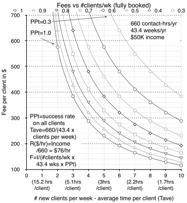
Figure 11.6: Number of clients versus minimum fee for measured success rate and average time per new client.
Figure 11.6 illustrates the flat rate equation 11.5. It shows the minimum fee versus new clients for the two measured parameters, success rate and average time per new client. The number of clients needed per week is quite large for the parameters we chose. If you have half the number of clients that you were planning on, then the fee is going to have to be twice as much to give you the same income as before. For example, for a success rate of 0.6, and an average time per new client of 1.9 hours, we have to see 8 new clients a week (for a fee of $240). If we have only 4 clients a week, following the curve of PPt=0.6, we’d have to have a fee of $480 to have the same overall income.
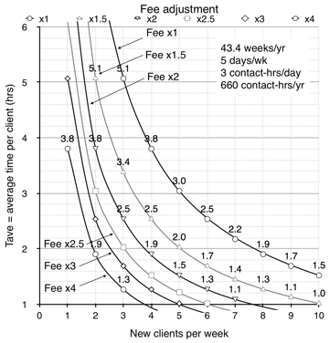
Figure 11.7: Plot of how much you have to multiply your fee if you don’t have a full client load (or get a lower income instead).
The upper right curve is for a full case-load at 660 contact-hours per year.
Figure 11.7 also illustrates the magnitude of the problem of needing new clients. You’ve optimized your fee for a full workload. Say your average time per new client (including diagnosis) is a fast 2.5 hours. This means you need to see an average of 6 new clients a week, every week you work that year to stay busy (the full client-load line is labeled Fee x1). But say you can only really average 3 new clients in the door a week? Well, you either earn half as much (6/3 = 0.5), or you have to double your fee to account for all the missed work. You can see this on the plot as the Fee x2 line.
- Example 11.12: How many clients do you need to meet your financial goals?
Let's compute how many clients the beginning therapist has to attract to his practice. From section 11.1, we’ll assume the typical private practice therapist has about W = 660 patient-contact hours per year. On average, this therapist has Pt = 80% of his clients continue after the diagnosis stage - these are the ones who he feels he can treat and who also choose to do therapy. Because our therapist is just a rookie, he is able to heal only P = 70% of them. (Thus, if he had 100 clients, 20 would have quit after diagnosis and 80 would have continued. Of that 80, Px80=56 would have healed and had a fee charged, and 24 would have not been helped fully and no fee would have been charged.) For this example, assume he spends T = 0.5 hours doing diagnosis and goal setting on every client who walks in the door, and he spends an additional average time of A = 2 hours per client he heals. He fails to heal 30% of the clients he has contracts with when he reaches his maximum cutoff time C = 3 hours. Thus:
Tave = 0.5 + 0.8 x 0.7 x 2 + 0.8 (1-0.7) 3
= 0.5 + 1.12 + 0.72
= 2.34 hours per client in the door
and the total number of clients per year needed would be:
NY = 660 hrs ÷ 2.34 hrs/client
= 282 new clients per year
Thus, given the assumptions in this example, the therapist spends on average 2.34 hours per new client in the door. If he has 660 client-contact hours, he would have to see 282 new clients (or returning clients with new issues) per year!
How does this work out on a weekly basis? Thus, for 43.4 weeks per year, he sees 282/43.4=6.5 new clients a week. This number is far larger than most therapists anticipate they will need.
Say the therapist decides to lower his fees (his fixed fee would be $317) by 10%, perhaps to be seen as more competitive. To get the same annual income he would have to work an additional 660 x 0.1 = 66 more hours per year and have an additional 282 x 0.1 = 28 clients to compensate (for the parameters of this example).
How much of an impact does one person have on the therapist’s income? If his target income was $50,000, and he computed his fees based on that, then each client that walks in the door impacts his total by $50,000 ÷ 282 = $177. Thus, for each additional client who comes in for a consultation, he gets on average only $177 (given our assumptions).
- Example 11.13: How many clients do you need now that you are more experienced?
Now, let us look at the same therapist after he's had more experience. Because he's gotten better at healing and evaluating clients, and not working with ones that he knows he can't help, his success rate healing clients has risen from 70% to P = 80%. But the percentage of clients in the door that he actually works with has gone down from 80% to Pt = 70%. He’s also able to diagnose quicker, so his average consult time in now T=0.4 hours. His average time to heal a client has gone up to A = 3 hours because he’s taking on tougher clients, and his cutoff time to quit trying to heal a client is C = 6 hours. He still has W = 660 contact-hours per year, and his target annual income is still $50K.
Tave = 0.4 + 0.7 x 0.8 x 3 + 0.7 x (1-0.8) x 6
= 0.5 + 1.68 + 0.84
= 3.02 hours per client in the door.
The total number of clients needed would be:
NY = 660 ÷ 3.02
= 219 clients per year.
Because the therapist takes more time per client on average, the therapist now needs to see 22% fewer clients than in Example 11.12 as one would expect. However, he has to raise his fee to compensate for the fact that he’s working slower, although getting more successes on average helps moderate this price increase. For an equivalent hourly rate of $76, his fixed fee would be $409.
His per client walking in the door income is now $50,000 ÷ 219 = $228.
For the fee he chose, he has to work a full caseload. Thus, he has to see 219/43.4=5 new clients per week. What happens if he can’t attract that many clients? His fee has to go up proportionally to the percentage of fewer clients per week. Say he can only average 3 new clients a week. His standard fee would have to go up 5/3 x $409 = $681 to have the same income. At this point, either he’s specializing so that clients think it is worth it, or he may have to specify a lower fee and take the reduced income.
Suggested Reading
- "Understanding 'Pay for Results' for Therapists". This is Chapter 3 from the
...or visit our Forum
Revision History
Sept 18, 2014: Put this supplement to appendix 10 from the Subcellular Psychobiology Diagnosis Handbook online.